Predictive models

What drives a professor’s rating — and can we predict who gets a ‘pepper’?

Questions 7 & 10

The regression here uses from-scratch OLS / ridge / lasso (numpy normal equations and coordinate descent), validated against scikit-learn in the test suite — the point is to show the math, not just call an API.

Q7 · Predicting rating from numeric features

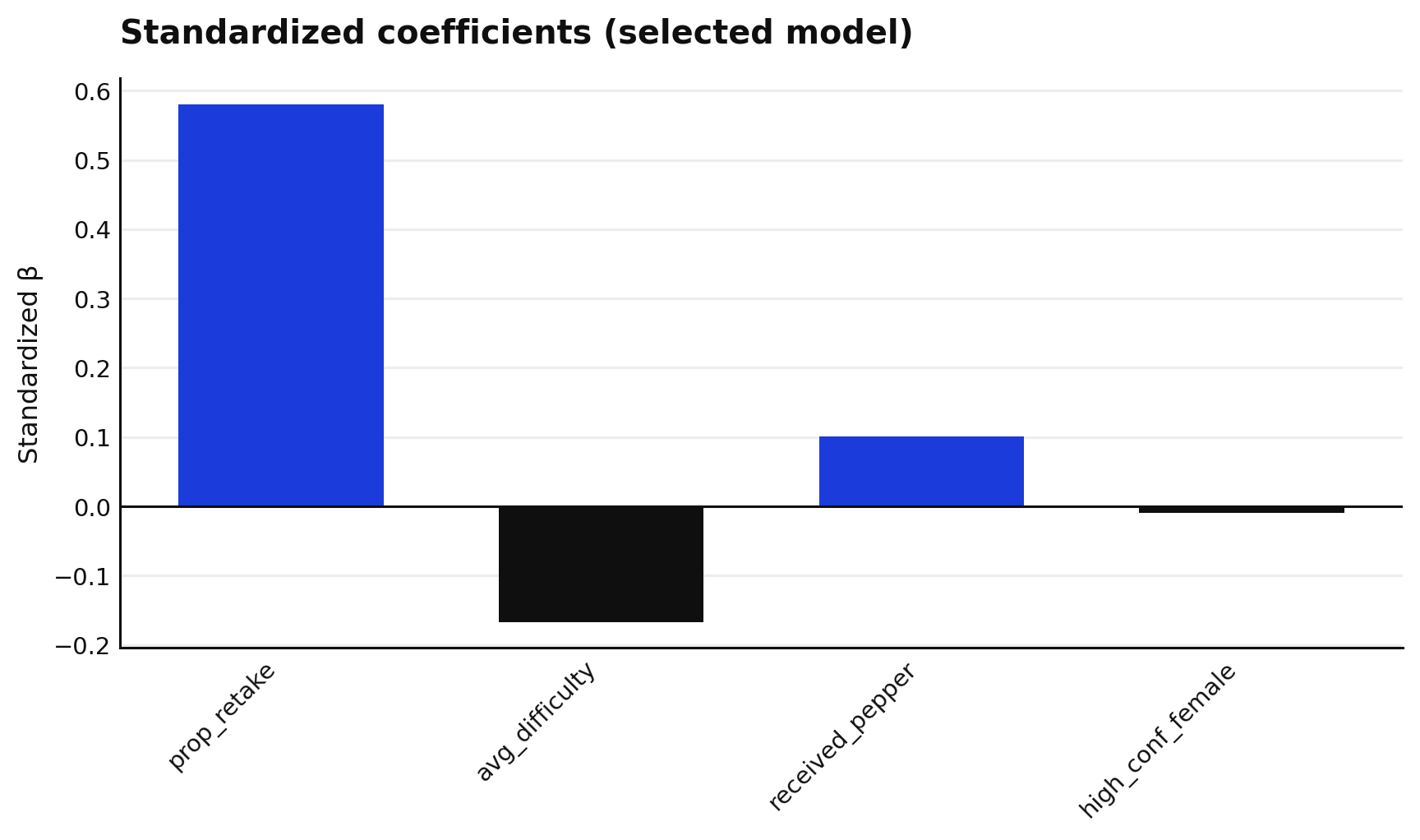
The question — Using only the numeric facts about a professor (difficulty, number of ratings, pepper, gender, online share, would-retake share), how well can we predict their rating, and what matters most?

How we answer it — Forward-select predictors with 5-fold cross-validation, then inspect the standardized coefficients of the chosen model.

Code

res, figs = questions.q7()
print("selected features:", ", ".join(res["best_features"]))
print(f"R² = {res['best_r2']:.3f}   RMSE = {res['best_rmse']:.3f}")
print(f"strongest predictor: {res['top_predictor']} (β = {res['top_predictor_beta']:.3f})")
show(figs, "q7_coefficients")

selected features: prop_retake, avg_difficulty, received_pepper, high_conf_female
R² = 0.810   RMSE = 0.356
strongest predictor: prop_retake (β = 0.581)

Figure 1: Standardized coefficients of the selected rating model.

Finding. A strong model (R² ≈ 0.81). The proportion of students who would retake the class dominates — on its own it explains ~77% of rating variance, which makes sense: “would you take them again?” is almost a restatement of “are they good?”. Difficulty and pepper add a little more.

Handling collinearity

“Would retake”, rating, and pepper are mutually correlated. Forward selection plus standardized coefficients keeps the model interpretable and avoids double-counting; ridge/lasso (in the package) give the same ranking with shrinkage.

Q10 · Predicting a “pepper”

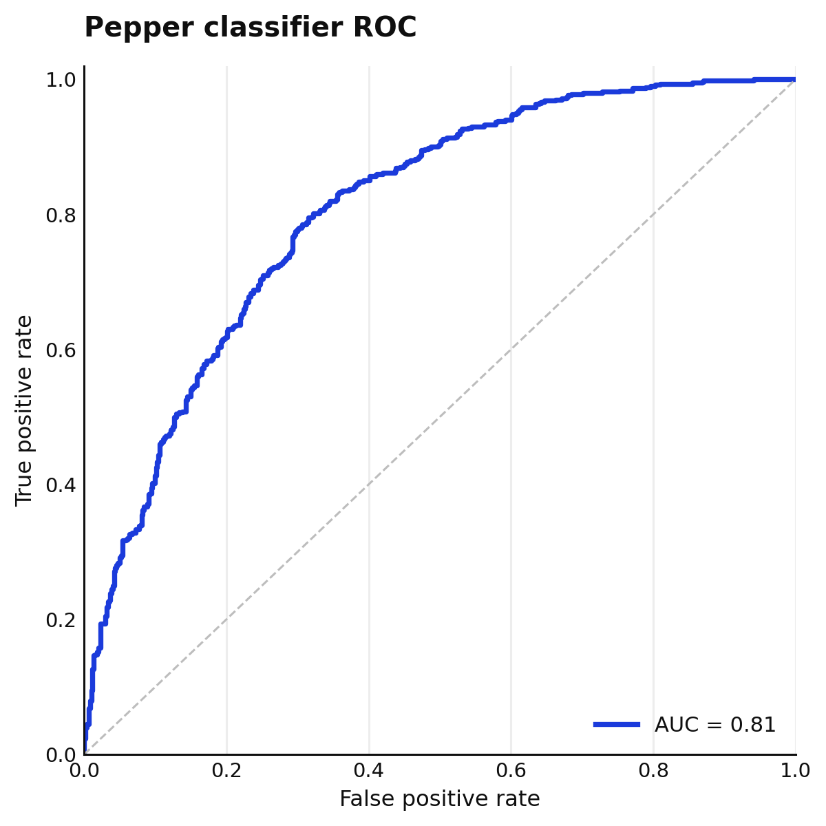
The question — Can we predict whether a professor is judged “hot” (a pepper) from everything we know — numeric features and tags?

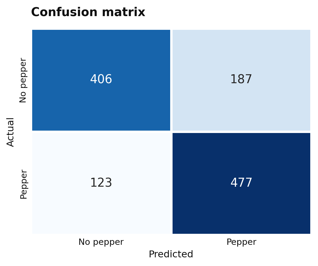
How we answer it — A class-balanced logistic-regression pipeline (standardization fit on the training folds only) over numeric + all 20 tags, evaluated by AUROC with a threshold chosen by Youden’s J.

Code

res10, figs10 = questions.q10()
print(f"n = {res10['n']}   pepper rate = {res10['pepper_rate']:.2f}")
print(f"AUC = {res10['auc']:.3f}   threshold (Youden J) = {res10['threshold']:.3f}")
print(f"F1: no-pepper = {res10['f1_class0']:.3f}, pepper = {res10['f1_class1']:.3f}")
show(figs10, "q10_roc")

n = 5963   pepper rate = 0.50
AUC = 0.805   threshold (Youden J) = 0.473
F1: no-pepper = 0.724, pepper = 0.755

Figure 2: ROC curve — AUC ≈ 0.81, an out-of-sample estimate.

Code

_, figs_cm = questions.q10()
show(figs_cm, "q10_confusion")

Figure 3: Confusion matrix at the Youden-J threshold.

Finding. A solid classifier (AUC ≈ 0.81). Average rating is the dominant signal — well-liked professors are much more likely to be marked “hot”. Because standardization is fit only on the training folds and the threshold comes from Youden’s J, this AUC is an honest out-of-sample estimate.

--- title: "Predictive models" subtitle: "What drives a professor's rating — and can we predict who gets a 'pepper'?" --- ```{python} #| label: setup #| echo: false import matplotlib.pyplot as plt from IPython.display import display from ape import questions def show(figs, *keys): """Display only the named figures; close the rest so nothing leaks.""" for k, f in figs.items(): if k not in keys: plt.close(f) for k in keys: display(figs[k]) plt.close("all") ``` [Questions 7 & 10]{.kicker} The regression here uses **from-scratch** OLS / ridge / lasso (numpy normal equations and coordinate descent), validated against scikit-learn in the test suite — the point is to show the math, not just call an API. ## Q7 · Predicting rating from numeric features ::: {.qbrief} **The question** — Using only the numeric facts about a professor (difficulty, number of ratings, pepper, gender, online share, would-retake share), how well can we predict their rating, and what matters most? **How we answer it** — Forward-select predictors with 5-fold cross-validation, then inspect the standardized coefficients of the chosen model. ::: ```{python} #| label: fig-q7 #| fig-cap: "Standardized coefficients of the selected rating model." res, figs = questions.q7() print("selected features:", ", ".join(res["best_features"])) print(f"R² = {res['best_r2']:.3f} RMSE = {res['best_rmse']:.3f}") print(f"strongest predictor: {res['top_predictor']} (β = {res['top_predictor_beta']:.3f})") show(figs, "q7_coefficients") ``` **Finding.** A strong model (**R² ≈ 0.81**). The **proportion of students who would retake the class** dominates — on its own it explains ~77% of rating variance, which makes sense: "would you take them again?" is almost a restatement of "are they good?". Difficulty and pepper add a little more. ::: {.callout-note collapse="true"} ## Handling collinearity "Would retake", rating, and pepper are mutually correlated. Forward selection plus standardized coefficients keeps the model interpretable and avoids double-counting; ridge/lasso (in the package) give the same ranking with shrinkage. ::: ## Q10 · Predicting a "pepper" ::: {.qbrief} **The question** — Can we predict whether a professor is judged "hot" (a pepper) from everything we know — numeric features *and* tags? **How we answer it** — A class-balanced logistic-regression **pipeline** (standardization fit on the training folds only) over numeric + all 20 tags, evaluated by **AUROC** with a threshold chosen by **Youden's J**. ::: ```{python} #| label: fig-q10-roc #| fig-cap: "ROC curve — AUC ≈ 0.81, an out-of-sample estimate." res10, figs10 = questions.q10() print(f"n = {res10['n']} pepper rate = {res10['pepper_rate']:.2f}") print(f"AUC = {res10['auc']:.3f} threshold (Youden J) = {res10['threshold']:.3f}") print(f"F1: no-pepper = {res10['f1_class0']:.3f}, pepper = {res10['f1_class1']:.3f}") show(figs10, "q10_roc") ``` ```{python} #| label: fig-q10-cm #| fig-cap: "Confusion matrix at the Youden-J threshold." _, figs_cm = questions.q10() show(figs_cm, "q10_confusion") ``` **Finding.** A solid classifier (**AUC ≈ 0.81**). Average rating is the dominant signal — well-liked professors are much more likely to be marked "hot". Because standardization is fit only on the training folds and the threshold comes from Youden's J, this AUC is an honest out-of-sample estimate.