Gender bias

Is there a pro-male bias in ratings — in the average, in the spread, and in perceived difficulty?

Questions 1–3, 5–6

Q1 · A pro-male bias in average rating?

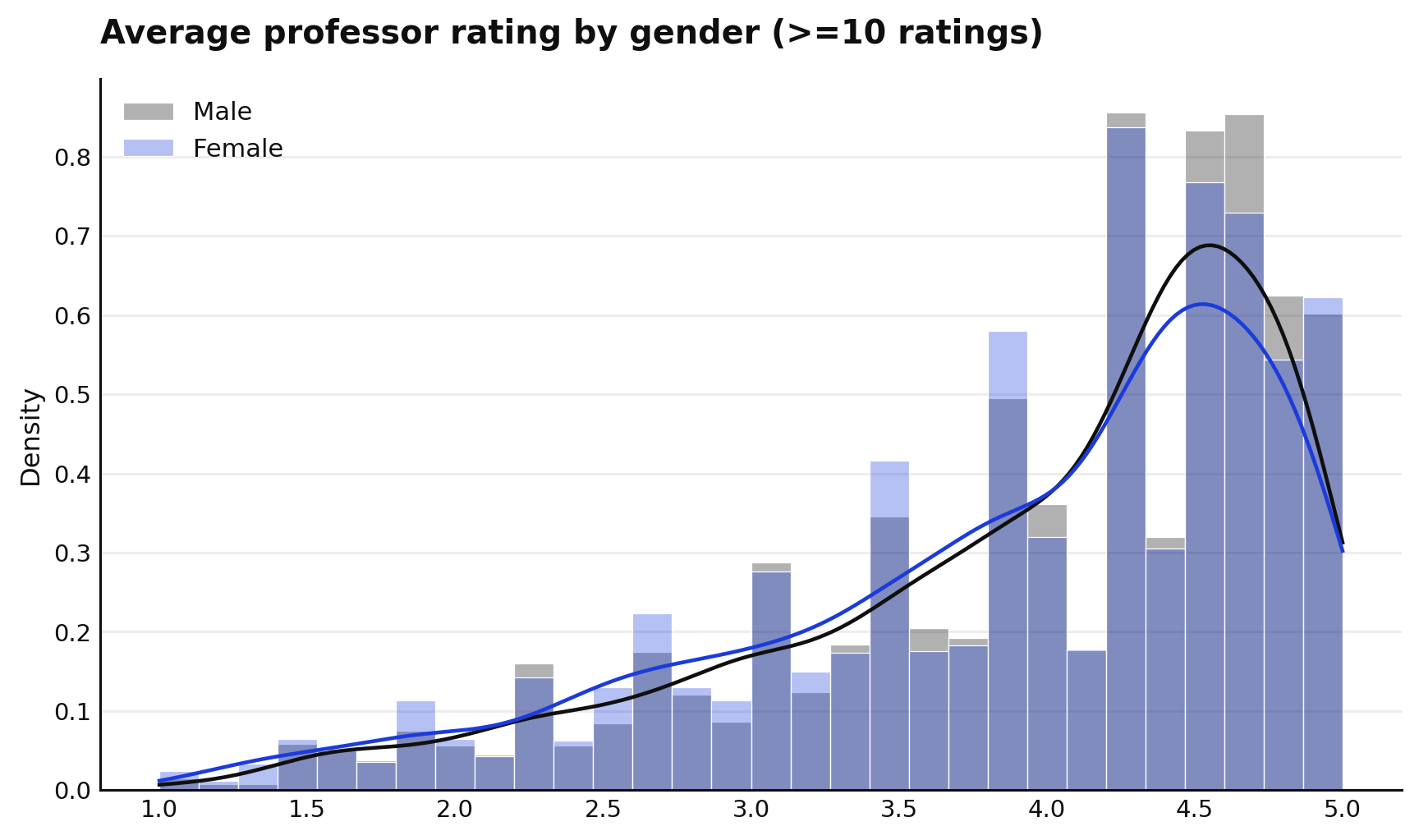
The question — Do students give male professors higher average ratings than female professors?

How we answer it — Compare the two rating distributions (professors with ≥ 10 ratings) with a one-sided Mann–Whitney U test (the claim is directional: men higher) and a Kolmogorov–Smirnov test.

Code

res, figs = questions.q1()
print(f"male mean   = {res['male_mean']:.3f}   (n={res['n_male']})")
print(f"female mean = {res['female_mean']:.3f}   (n={res['n_female']})")
print(f"Mann-Whitney U (one-sided, male>female): p = {res['mwu_p_one_sided_greater']:.2e}")
print(f"KS test: p = {res['ks_p']:.2e}")
show(figs, "q1_rating_by_gender")

male mean   = 3.964   (n=3987)
female mean = 3.889   (n=3118)
Mann-Whitney U (one-sided, male>female): p = 3.65e-04
KS test: p = 2.77e-03

Figure 1: Rating distributions overlap heavily; men’s mean sits slightly higher.

Finding. Men average ≈ 3.96 vs. women ≈ 3.89 — a statistically significant pro-male gap (p ≈ 4 × 10⁻⁴ < 0.005). “Significant” is not the same as “large”, though — see Q3.

Why this test

Ratings are bounded (1–5) and skewed, so we use rank-based non-parametric tests rather than a t-test. Because the hypothesis is directional, we use a one-sided test, and we estimate the gap on the full ≥ 10-rating sample rather than slicing into many subgroups.

Q2 · A difference in the spread of ratings?

The question — Even if the averages are close, are women’s ratings more polarised (more spread out) than men’s?

How we answer it — Compare the variance of the two distributions with Levene’s test.

Code

res2, _ = questions.q2()
print(f"male variance   = {res2['male_var']:.3f}")
print(f"female variance = {res2['female_var']:.3f}")
print(f"Levene's test: p = {res2['levene_p']:.4f}  ->  {'different' if res2['significant'] else 'not different'}")
plt.close("all")

male variance   = 0.735
female variance = 0.807
Levene's test: p = 0.0024  ->  different

Finding. Women’s ratings are more dispersed (variance 0.81 vs. 0.74); Levene’s test is significant (p ≈ 0.002). Spread is a different question from the average — hence a variance test.

Q3 · How big are these effects?

The question — If a pro-male gap and a spread difference exist, how large are they in practical terms?

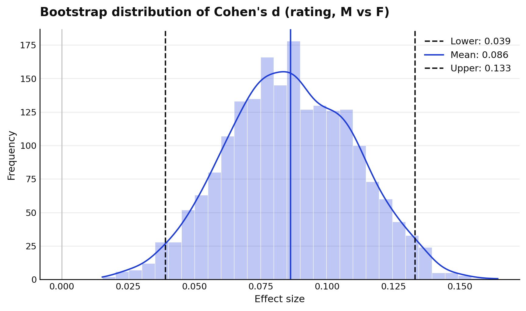
How we answer it — Estimate Cohen’s d (the standardized mean gap) and the variance ratio (spread), each with a 95% bootstrap confidence interval.

Code

res3, figs3 = questions.q3()
print(f"Cohen's d (rating, M vs F) = {res3['cohen_d']:.3f}  95% CI {tuple(round(x,3) for x in res3['cohen_d_ci'])}")
print(f"Variance ratio (M/F)       = {res3['variance_ratio']:.3f}  95% CI {tuple(round(x,3) for x in res3['variance_ratio_ci'])}")
show(figs3, "q3_effect_size")

Cohen's d (rating, M vs F) = 0.086  95% CI (np.float64(0.039), np.float64(0.133))
Variance ratio (M/F)       = 0.911  95% CI (np.float64(0.849), np.float64(0.98))

Figure 2: Bootstrap distribution of Cohen’s d for the rating gap; the 95% CI sits above zero but the effect is small.

Finding. The mean effect is small — Cohen’s d ≈ 0.09 (95% CI just above 0). The variance ratio ≈ 0.91 (CI below 1) confirms women’s wider spread. The honest takeaway: a real but small pro-male bias in the average, and a small difference in spread.

Q5 · A gender difference in difficulty?

The question — Do students perceive female professors as harder (or easier) to take than male professors?

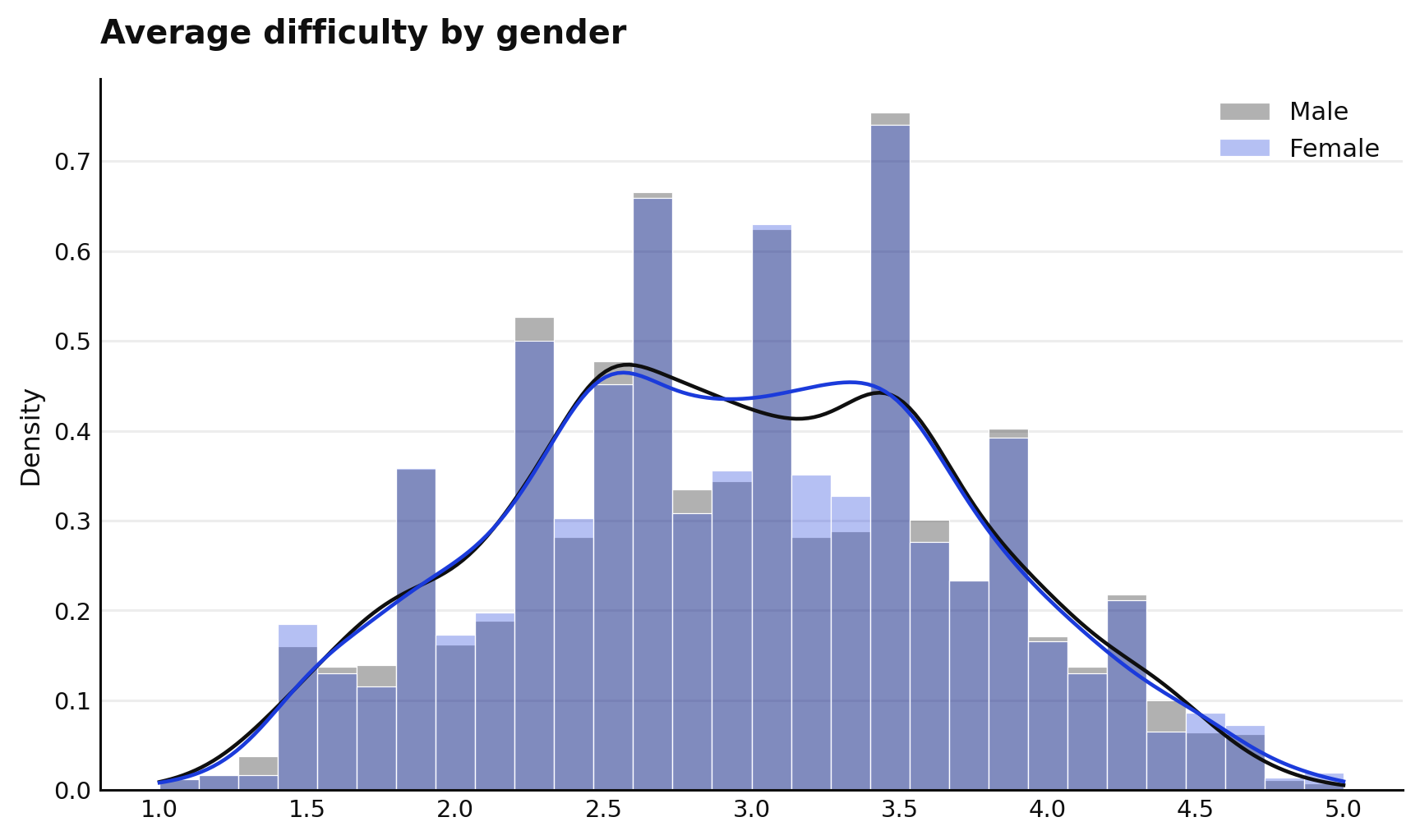
How we answer it — Compare the average-difficulty distributions by gender (Mann–Whitney U + KS).

Code

res5, figs5 = questions.q5()
print(f"male mean difficulty   = {res5['male_mean']:.3f}")
print(f"female mean difficulty = {res5['female_mean']:.3f}")
print(f"Mann-Whitney U: p = {res5['mwu_p']:.3f}   KS: p = {res5['ks_p']:.3f}")
show(figs5, "q5_difficulty_by_gender")

male mean difficulty   = 2.940
female mean difficulty = 2.947
Mann-Whitney U: p = 0.786   KS: p = 0.997

Figure 3: Difficulty distributions are essentially identical across genders.

Finding. No difference (p ≈ 0.79). Students rate male and female professors as equally difficult.

Q6 · How big is the difficulty difference?

The question — Putting a number on the (non-)difference in difficulty.

How we answer it — Cohen’s d on difficulty, with a 95% bootstrap CI.

Code

res6, _ = questions.q6()
print(f"Cohen's d (difficulty) = {res6['cohen_d']:.3f}  95% CI {tuple(round(x,3) for x in res6['cohen_d_ci'])}")
plt.close("all")

Cohen's d (difficulty) = -0.009  95% CI (np.float64(-0.058), np.float64(0.039))

Finding. d ≈ 0 with a CI straddling zero — a clean null, where the effect size and its interval agree there is nothing there.

--- title: "Gender bias" subtitle: "Is there a pro-male bias in ratings — in the average, in the spread, and in perceived difficulty?" --- ```{python} #| label: setup #| echo: false import matplotlib.pyplot as plt from IPython.display import display from ape import questions def show(figs, *keys): """Display only the named figures; close the rest so nothing leaks.""" for k, f in figs.items(): if k not in keys: plt.close(f) for k in keys: display(figs[k]) plt.close("all") ``` [Questions 1–3, 5–6]{.kicker} ## Q1 · A pro-male bias in average rating? ::: {.qbrief} **The question** — Do students give male professors higher average ratings than female professors? **How we answer it** — Compare the two rating distributions (professors with ≥ 10 ratings) with a *one-sided* Mann–Whitney U test (the claim is directional: men higher) and a Kolmogorov–Smirnov test. ::: ```{python} #| label: fig-q1 #| fig-cap: "Rating distributions overlap heavily; men's mean sits slightly higher." res, figs = questions.q1() print(f"male mean = {res['male_mean']:.3f} (n={res['n_male']})") print(f"female mean = {res['female_mean']:.3f} (n={res['n_female']})") print(f"Mann-Whitney U (one-sided, male>female): p = {res['mwu_p_one_sided_greater']:.2e}") print(f"KS test: p = {res['ks_p']:.2e}") show(figs, "q1_rating_by_gender") ``` **Finding.** Men average ≈ 3.96 vs. women ≈ 3.89 — a **statistically significant** pro-male gap (p ≈ 4 × 10⁻⁴ < 0.005). "Significant" is not the same as "large", though — see Q3. ::: {.callout-note collapse="true"} ## Why this test Ratings are bounded (1–5) and skewed, so we use **rank-based** non-parametric tests rather than a t-test. Because the hypothesis is directional, we use a **one-sided** test, and we estimate the gap on the full ≥ 10-rating sample rather than slicing into many subgroups. ::: ## Q2 · A difference in the *spread* of ratings? ::: {.qbrief} **The question** — Even if the averages are close, are women's ratings more polarised (more spread out) than men's? **How we answer it** — Compare the variance of the two distributions with Levene's test. ::: ```{python} #| label: q2 res2, _ = questions.q2() print(f"male variance = {res2['male_var']:.3f}") print(f"female variance = {res2['female_var']:.3f}") print(f"Levene's test: p = {res2['levene_p']:.4f} -> {'different' if res2['significant'] else 'not different'}") plt.close("all") ``` **Finding.** Women's ratings are **more dispersed** (variance 0.81 vs. 0.74); Levene's test is significant (p ≈ 0.002). Spread is a different question from the average — hence a variance test. ## Q3 · How big are these effects? ::: {.qbrief} **The question** — If a pro-male gap and a spread difference exist, how large are they in practical terms? **How we answer it** — Estimate **Cohen's d** (the standardized mean gap) and the **variance ratio** (spread), each with a 95% bootstrap confidence interval. ::: ```{python} #| label: fig-q3 #| fig-cap: "Bootstrap distribution of Cohen's d for the rating gap; the 95% CI sits above zero but the effect is small." res3, figs3 = questions.q3() print(f"Cohen's d (rating, M vs F) = {res3['cohen_d']:.3f} 95% CI {tuple(round(x,3) for x in res3['cohen_d_ci'])}") print(f"Variance ratio (M/F) = {res3['variance_ratio']:.3f} 95% CI {tuple(round(x,3) for x in res3['variance_ratio_ci'])}") show(figs3, "q3_effect_size") ``` **Finding.** The mean effect is **small** — Cohen's d ≈ 0.09 (95% CI just above 0). The variance ratio ≈ 0.91 (CI below 1) confirms women's wider spread. The honest takeaway: a *real but small* pro-male bias in the average, and a small difference in spread. ## Q5 · A gender difference in *difficulty*? ::: {.qbrief} **The question** — Do students perceive female professors as harder (or easier) to take than male professors? **How we answer it** — Compare the average-difficulty distributions by gender (Mann–Whitney U + KS). ::: ```{python} #| label: fig-q5 #| fig-cap: "Difficulty distributions are essentially identical across genders." res5, figs5 = questions.q5() print(f"male mean difficulty = {res5['male_mean']:.3f}") print(f"female mean difficulty = {res5['female_mean']:.3f}") print(f"Mann-Whitney U: p = {res5['mwu_p']:.3f} KS: p = {res5['ks_p']:.3f}") show(figs5, "q5_difficulty_by_gender") ``` **Finding.** **No** difference (p ≈ 0.79). Students rate male and female professors as equally difficult. ## Q6 · How big is the difficulty difference? ::: {.qbrief} **The question** — Putting a number on the (non-)difference in difficulty. **How we answer it** — Cohen's d on difficulty, with a 95% bootstrap CI. ::: ```{python} #| label: q6 res6, _ = questions.q6() print(f"Cohen's d (difficulty) = {res6['cohen_d']:.3f} 95% CI {tuple(round(x,3) for x in res6['cohen_d_ci'])}") plt.close("all") ``` **Finding.** d ≈ 0 with a CI straddling zero — a clean null, where the effect size *and* its interval agree there is nothing there.